Signal Processing Know-How
Types of Synchronous Measurement
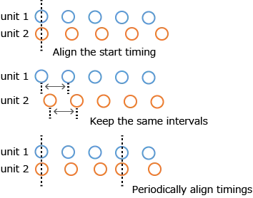
Synchronous measurement refers to the measurement of multiple signals with equal timing. Note that there are various definitions of equal timing.
- Aligning the start timing.
- Aligning the measurement interval by aligning the internal clocks of the measuring instrument.
- Periodically correcting timing errors.
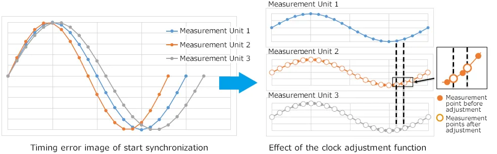
Since AirLogger™ operates measurement units by wireless communication, the PC communication unit periodically sends out a synchronous signal to align the measurement timing between measurement units. (For 100 ms sampling or more)
For high-speed sampling of 50 ms or less, AirLogger™ sends out a synchronous signal to align the start timing.
The standard software of WM2000 series has a clock adjustment function, to correct the clock using the start and stop timings for high-speed sampling by post-measurement calculation. By using the clock adjustment function , the measurement timing between measurement units can be aligned.
Sampling Frequency (Period) and Signal Frequency (Period) ~ Twice the sampling is not enough ~
The sampling theorem gives the impression that sampling at twice the frequency may not be a problem, however, as far as can be directly seen in the waveform from measurement with a data logger, the number of data is not enough.
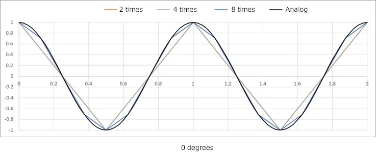
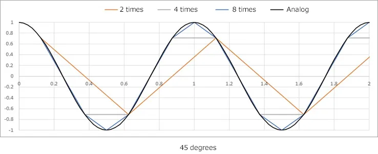
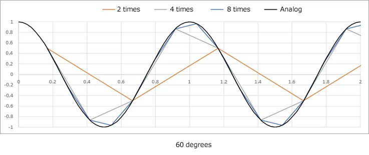
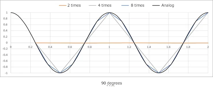
The figure shows waveforms when a sine wave (cosine wave) with a frequency of 1 Hz (period of 1 s) is sampled at 2 times, 4 times, and 8 times higher frequency.
When the phase is changed to 45, 60, and 90 degrees, the waveform becomes as shown in the figure.
The waveform will change depending on the phase up to 4 times the frequency.
It takes more than 8 times frequency to capture a waveform with good visual reproduction.
In addition, if the signal contains a higher harmonic wave such as pulses and the waveform is sharply angled, it becomes even more difficult to extract the apex.
*The sampling theorem is twice the highest frequency, NOT twice the waveform repetition frequency.
Sampling with 10 times the signal frequency and using a low-pass filter with a cutoff frequency of 1/10 of the sampling frequency will give stable results since high frequency components are curbed by the filter.
Sampling and Waveform Reproduction
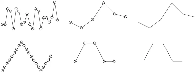
A signal takes continuous values, but the measured values are taken as a discrete values corresponding to the sampling frequency, and the waveform is displayed as a line connecting the discrete values.
As shown in the figure below, if the result of measurement at 21 points is thinned out to 5 points by a quarter, the waveform appears as a different waveform.
The sampling frequency should be notably higher than the frequency component of the signal to be measured.
This is especially true for the peak of a triangular wave.
The fewer the number of sampling, the more the lack of apexes.
If the signal has a low frequency and produces a high frequency noise, by thinning out the measured value derived from the measurement, which is performed at a higher sampling frequency and with a low-pass filter, which makes waveform gently curved, a highly reproducible signal can be measured.
Frequency noises can be removed by digital filter functions of AirLogger™ standard software after measurement using this software. There are thinning functions that increase the sampling period in order to reduce the number of measurement points.
Using these two functions, the signal frequency of the measured value can be limited and stable measurement results can be obtained.
For more information, please refer to “Usage Handbook: Digital Filter”.
For more information, please refer to “Usage Handbook: Decimation after Measurement”.
Extracting Only the Amplitude Information (AM Detection, Envelope Detection)
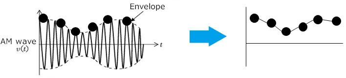
Extracting only the amplitude of an AC signal can be achieved by using AM detection.
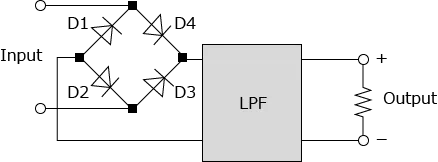
A simple AM detection circuit can be made possible using a full-wave rectifier circuit and a low-pass filter as shown in the figure.
AM detection can be easily achieved by arithmetic operations:
- Capturing the signal with the value converted by the formula of the square root of square
- Applying a low-pass filter to the measurement result
These two steps result in a waveform with only the amplitude information.
After converting to the amplitude information only, the sampling period can be reduced.
By thinning out the converted measurement results, the data can be lightened and handled.
How To Input Conversion, Correction Equations and Types of Functions,
How To Compute with Measurement Values of Different Channels: Multi-channel Calculation Function,
Digital Filter, and Decimation after Measurement in the Usage Handbook.
How to Show 2-way Value Display
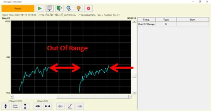
In AirLogger™, when an out-of-range voltage is input, the output value will be displayed as “Out Of Range”.
| NAME | Sensor3-1 |
|---|---|
| 0 | Out of Range |
| 1 | Out of Range |
| 2 | Out of Range |
| 3 | Out of Range |
| 4 | -5.28 |
| 5 | -5.13 |
| 6 | -5.15 |
| 7 | -5.13 |
| 8 | -4.8 |
| 9 | Out of Range |
| 10 | Out of Range |
| 11 | Out of Range |
| 12 | Out of Range |
| 13 | Out of Range |
| 14 | -5.13 |
| 15 | -5.04 |
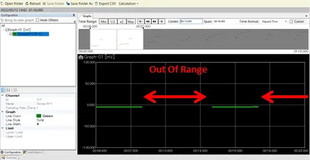
By inputting pulse voltages above the set range within the maximum absolute rated voltage and using 0V and “Out Of Range” will allow gates to be displayed in the log.
In a CSV file, “Out Of Range” can be changed to any character by replacing the character in the file with the desired one.
Example
| NAME | Sensor3-1 |
|---|---|
| 0 | Under test |
| 1 | Under test |
| 2 | Under test |
| 3 | Under test |
| 4 | -5.28 |
| 5 | -5.13 |
| 6 | -5.15 |
| 7 | -5.13 |
| 8 | -4.8 |
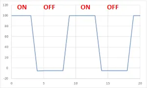
(Numeric values make it easy to overwrite them on a separately created characteristic graph.)
“Out of Range” -> 100
Digital Filter
Noise is added to the signal in the measurement data. Filters are used to remove only the noise without changing the signal.
There are various types of filters.
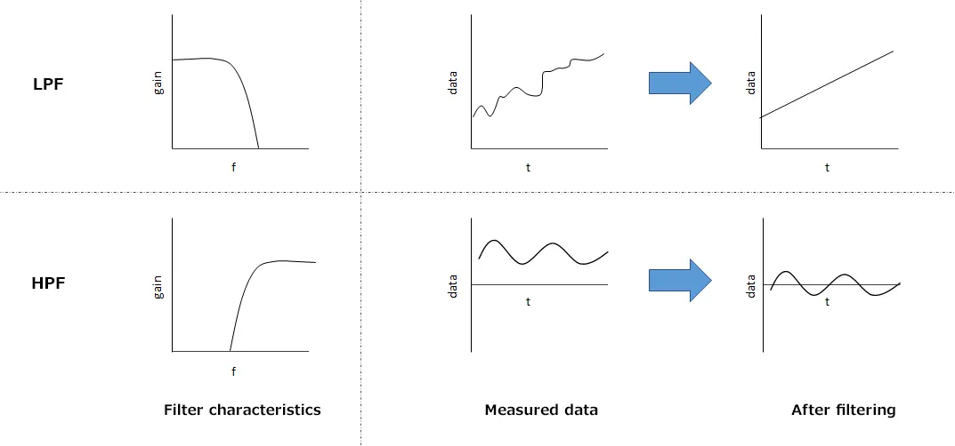
Low-pass filters (LPF) and high-pass filters (HPF) are commonly used.
These two types of filters remove frequencies higher (LPF) or lower (HPF) than the specified frequency (cutoff frequency).
The LPF removes data with frequencies above the cutoff frequency. When viewed as a time waveform, it removes flickering noises, resulting in a smooth waveform.
The HPF removes data with frequencies below the cutoff frequency. When viewed as a time waveform, it removes noises such as offset data and slowly moving fluctuations.
A filter that is realized by digital data processing is called a digital filter.
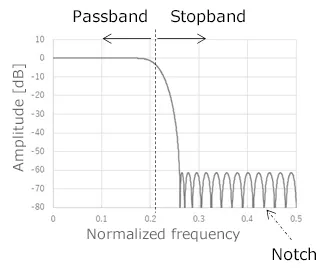
The characteristics of an LPF made of a digital filter are shown in the figure.
In general, the characteristics of the stopband have recurring peaks, and the frequency at which the amplitude becomes zero is called as the notch frequency.
The simplest digital filter is a moving average filter that uses the average of the data adjacent to back and forth.
The filter characteristic of the moving average is a sinc function in the LPF.
The notch frequency depends on the range over which the average is taken.
(For a moving average of 10 data in 1 s sampling, the notch frequency is an integer multiple of 0.1 Hz.)
The FIR filter designed by the Parks-McClellan algorithm is used in the WM2000 standard software.
For details on how to use the filter, please refer to the “Filter Operations” section of the User’s Manual or “Digital Filter” linked below:
Noise Removal Methods for Commercial Frequency
Noise affected by AC power supply may have a large value.
Since the frequency of the AC power supply is fixed, a filter with a high removal rate only for that frequency is required.
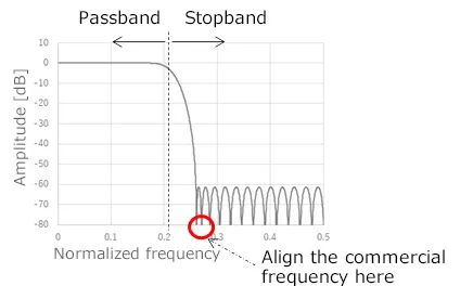
Digital filters have a notch in the stopband.
By matching the notch frequency to the frequency of the AC power supply, significant noise removal can be easily achieved.
The notch frequency depends on the sampling period, the number of samplings, and the type of filter of the digital filter.
How to Simultaneously Extract Measured Raw Data and Results Using A Conversion Formula (Multi-data Calculation Function)
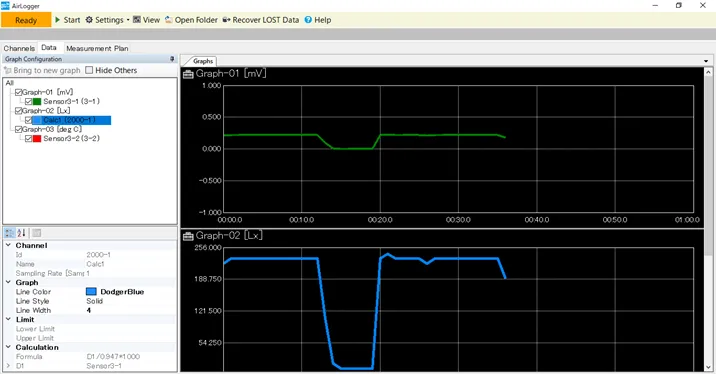
The results of calculated measured values using conversion formulas can be output in the WM2000 series.
When results are extracted using the normal conversion formula, only the results after conversion can be checked, whereas the results before conversion may not be viewed.
By using the multi-data calculation function, which is designed to perform calculations using multiple measurement values, it is possible to simultaneously display the data before and after the conversion.
A single channel calculation can also be registered using the multi-data calculation function.
The result of using an illuminance sensor to display the sensor output voltage and the converted illuminance can be displayed as shown in the below graphs.
Usage Handbook: How To Compute with Measurement Values of Different Channels: Multi-channel Calculation Function